The Relational Workflow Model¶

The Relational Workflow Model interprets tables as workflow steps, rows as workflow artifacts, and foreign keys as execution order. The schema specifies not only what data exists but how it is derived — a single formal system in which data structure, computational dependencies, and integrity constraints are all queryable, enforceable, and machine-readable. This unification is what makes DataJoint a computational substrate rather than a database in the conventional sense. The worked example below shows the model in action; its place in the lineage of relational modeling follows.

A worked example¶

Diagrams in this documentation use the same notation as dj.Diagram in datajoint-python: Manual tables are green rounded boxes, Lookup tables are gray rounded boxes, Imported tables are blue ellipses, and Computed tables are orange ellipses. A Part table is a small plain box grouped with its master inside a light box (the entity cluster). Tier is conveyed by shape and color, and edge thickness shows how a child relates to its parent — a thick line means the child extends the parent (one per parent); a thin line means the child is contained within the parent (many per parent). Edges are drawn without arrowheads, so direction is read from the layout. 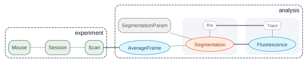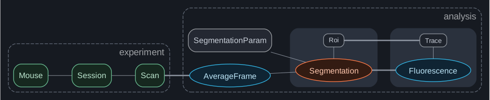A diagram uses a single orientation throughout — either left-to-right or top-to-bottom — and which one is usually obvious at a glance. This one is left-to-right, so every foreign key points from an upstream table on the left to the downstream table that depends on it on the right (a top-to-bottom diagram reads the same way, upstream at the top). The one exception is a master–part group: a Part is drawn level with its master rather than downstream of it, but a part's foreign key always references its master, so the part is always downstream. They are placed together because a master and its parts are always populated in a single transaction. Tables are grouped into their schemas — the labeled boxes — and dependencies cross schema boundaries freely. 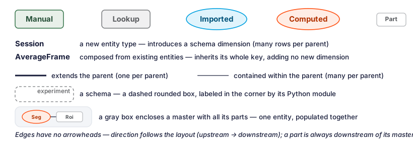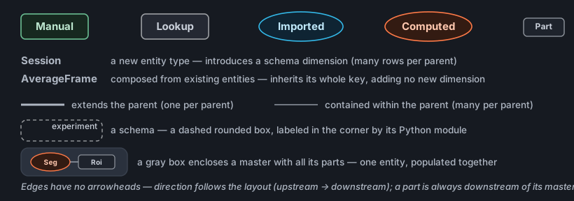An underlined name marks a new entity type — the table introduces a new key attribute, a new schema dimension, so it holds many rows per parent — while a plain name is composed from existing entities, extending one or combining several, inheriting its whole key and adding no new dimension. The legend below the figure keys the full notation.

Worked-example imaging pipeline diagram spanning two schemas: experiment (Mouse → Session → Scan) and analysis (AverageFrame → Segmentation → Fluorescence, with Lookup SegmentationParam feeding Segmentation, and the Part tables Roi on Segmentation and Trace on Fluorescence).

The notation is specified in full in the Diagram specification. The concepts it depicts are explained in depth elsewhere: entity integrity (keys, entity types, and schema dimensions), master–part tables (the entity group and its all-or-nothing populate), the computation model (how make() produces Imported and Computed tables), and semantic matching (why a name means the same thing everywhere it appears).

The pipeline spans two schemas: experiment holds the raw, manually entered tables, and analysis holds everything derived from them. Mouse, Session, and Scan are Manual tables entered by the experimenter. SegmentationParam is a Lookup table holding reference parameter sets. AverageFrame is Imported — its make() reads the TIFF identified by Scan (a dependency reaching across from experiment into analysis) and stores the mean fluorescence frame. Segmentation is Computed — its primary key fans in from both AverageFrame and SegmentationParam, so every average frame is segmented with every parameter set automatically; its Part table Roi holds the individual regions found in each segmentation. Fluorescence then extracts per-ROI time-series from each segmentation, and its Part table Trace stores one trace per region — each Trace row tied back to the Roi it measures. A master and its parts form one entity, inserted and deleted together. No external scheduler is consulted: the foreign-key graph dictates what may run, what must run first, and what already exists. The pipeline DAG and the database schema are the same object.

Three interpretations of the relational model¶

The relational model has historically admitted two interpretations. Codd's mathematical foundation (1970) views tables as logical predicates and rows as true propositions — rigorous but abstract. Chen's Entity-Relationship Model (1976) views tables as entity types or relationships — intuitive for domain modeling, but silent on how entities come into being. The Relational Workflow Model adds a third, the one the worked example above illustrates.

Aspect	Mathematical (Codd)	Entity-Relationship (Chen)	Relational Workflow (DataJoint)
Core question	What functional dependencies exist?	What entity types exist?	When and how are entities created?
Table semantics	Logical predicate	Entity or relationship	Workflow step
Row semantics	True proposition	Entity instance	Workflow artifact
Foreign keys	Referential integrity	Relationship	Execution order
Computation	Not addressed	Not addressed	Declared in schema
Data lineage	Not addressed	Not addressed	Structural
Implementation gap	High	High	None

A semantic interpretation, not a departure¶

The Relational Workflow Model layers a semantic interpretation on the classical relational model; it does not replace any of it. Tables, rows, primary and foreign keys, normalization, and the query algebra keep their classical meaning. The model adds four readings on top:

Tables also represent workflow steps.
Rows also represent workflow artifacts, traceable to their inputs.
Foreign keys also prescribe execution order — the dependency graph is the pipeline DAG, enforced by the database.
Computed and Imported tables carry their own make() methods, declaring derivation logic in the schema itself rather than in an external workflow file.

Under this interpretation the schema becomes active. A row exists in a Computed table if and only if its upstream key exists, its make() has run, and its result satisfies the declared constraints. The schema is the executable specification of the work.

The deliberate trade-off¶

DataJoint accepts tighter coupling deliberately, in exchange for one formal system that spans data structure, computation, dependencies, and integrity. See Comparison to Workflow Languages for the structural treatment — what file-based workflows and task orchestrators each offer, what each omits, and when to use them alongside DataJoint.

Substrate consequences¶

Because dependencies are declared before any computation runs, lineage and reproducibility become properties of the substrate, not artifacts assembled after the fact. Every row in Segmentation is reachable by foreign key from the exact AverageFrame and SegmentationParam that produced it; cascade deletes remove dependent results when their inputs become invalid. Reproducibility is structural rather than retrofitted by audit: a computed result cannot exist without its upstream entities, and the declared types and constraints must hold. The model enforces what other systems merely log. The lineage graph is already in the schema; mapping it to external standards such as W3C PROV or OpenLineage is a translation, not a reconstruction.

The same property makes the schema a shared contract between humans and the machines that increasingly collaborate with them. The schema is self-describing: an agent can introspect table structure, dependencies, and state programmatically. Operations are safe by default: invalid joins, type mismatches, and referential violations fail cleanly rather than corrupting data silently. The dependency graph is explicit: agents reason about execution order without implicit knowledge. Core operations are idempotent: retries on failure are without side effects. And all state — job status, computation progress, errors — is queryable, so the work is observable as it happens. These are the properties that let agents participate in scientific workflows with the same transactional guarantees that protect human-initiated work.

Beneath the model¶

The remaining sections detail the structural elements that make the model work in practice.

Workflow steps and table tiers¶

Tables are classified into tiers by data-entry mode:

Tier	Role	`make()`
Manual	Rows entered at runtime from outside the pipeline (people, forms, instruments, imports)	No
Lookup	Reference rows defined in the schema itself via `contents`	No
Imported	Reach out to data sources outside DataJoint (instruments, ELNs, external databases)	Yes
Computed	Derive their contents entirely from upstream DataJoint tables	Yes

Imported and Computed tables define computations via make() methods. The make() method specifies how each entity is derived — declared within the table definition, not in an external workflow file.

Manual vs. Lookup¶

Manual and Lookup tables are both entry points — their rows are entered rather than derived by a make() — but they differ in where the rows come from:

A Manual table's rows arrive at runtime, from outside the pipeline: a person typing into a form, a LIMS, an instrument, or an import from another system. Its contents are specific to a particular project or experiment and differ from one deployment to the next. Manual tables are the pipeline's origin points — e.g. Mouse, Session, Scan.
A Lookup table's rows are part of the schema definition, declared in code through the contents attribute and versioned alongside the table. Its contents are the same wherever the schema is deployed and change only when the code changes. Use it for reference values that belong to the pipeline's design: parameter sets, method definitions, controlled vocabularies, enumerations — e.g. SegmentationParam.

The quick test is where does a row come from? If it is fixed in the committed schema (contents), it is a Lookup; if it arrives at runtime, it is a Manual table. A common mistake is to use a Lookup for data that is actually entered at runtime (for example, filled in through a dashboard form). If a table's rows do not come from its committed contents, it belongs in the Manual tier.

Because Lookup content lives in the code, changing it is a code change: you edit contents and redeploy, so updates flow through the same review-and-deploy (CI/CD) process as any other schema change — versioned and reproducible across deployments. Manual content, by contrast, is entered at runtime and never touches the codebase.

Master-part relationships¶

Master-part relationships declare transactional grouping directly in the schema. The master table represents the workflow step; part tables hold the items produced together. Insertions and deletions cascade as a unit, enforcing transactional semantics without application code.

Workflow normalization¶

"Every table represents an entity type created at a specific workflow step, and all attributes describe that entity as it exists at that step."

Classical normalization theory decomposes tables to eliminate redundancy through normal forms based on functional dependencies. Entity normalization asks whether each attribute describes the entity identified by the primary key. Workflow normalization extends these principles with a temporal dimension: each table's attributes must describe its entity as it exists at the workflow step the table represents. A Session table holds attributes known when the session is entered (date, experimenter, subject); analysis parameters determined later belong in Computed tables that depend on Session. The discipline prevents tables that accumulate attributes from different workflow stages, obscuring lineage and complicating updates.

Entity integrity¶

All data is represented as well-formed entity sets with primary keys identifying each entity uniquely. When upstream data is deleted, dependent results cascade-delete automatically — including associated objects in external storage. To correct errors, you delete, reinsert, and recompute, ensuring every result represents a consistent computation from valid inputs.

Query algebra and algebraic closure¶

DataJoint provides a five-operator algebra:

Operator	Symbol	Purpose
Restrict	`&`	Filter entities by attribute values or membership in other relations
Project	`.proj()`	Select and rename attributes, compute derived values
Join	`*`	Combine related entities across relations
Aggregate	`.aggr()`	Group entities and compute summary statistics
Union	`+`	Combine entity sets with compatible structure

The algebra achieves algebraic closure: every operator produces a valid entity set with a well-defined primary key, enabling unlimited composition. This preservation of entity integrity — every query result is itself a proper entity set with clear identity — distinguishes DataJoint's algebra from SQL, where query results lack both a well-defined primary key and a clear entity type.

Two readings of the same schema¶

The classical relational reading and the workflow reading hold simultaneously — they are interpretive lenses on the same schema, not incompatible designs.

Classical reading	Workflow reading
Tables store data	Tables represent workflow steps
Rows are records	Rows are workflow artifacts
Foreign keys enforce consistency	Foreign keys prescribe execution order
Updates modify state	Computations create new states
Schemas organize storage	Schemas specify pipelines
Queries retrieve data	Queries trace lineage